How the Radial Panel Logic Works in Grasshopper
A technical follow-up to the Rapperswil Castle canopy study
In the previous post, I described the replacement study for the funnel-shaped textile canopy in the courtyard of Rapperswil Castle and discussed why a radial panel layout became essential. This follow-up explains the technical side of that process in more detail: how the helper geometry is built in Rhino, how the workflow is structured in Grasshopper, and why the core logic is best handled inside a C# script component.
The purpose of this post is not to present a software trick. It is to make the method itself understandable. The workflow is only useful if the geometry, the logic, and the limits of the script are all transparent.
What the script is meant to do
The script does not generate the final cutting pattern. It generates a helper geometry.
The task is the following:
take a closed boundary curve
define an internal reference point
define a start direction
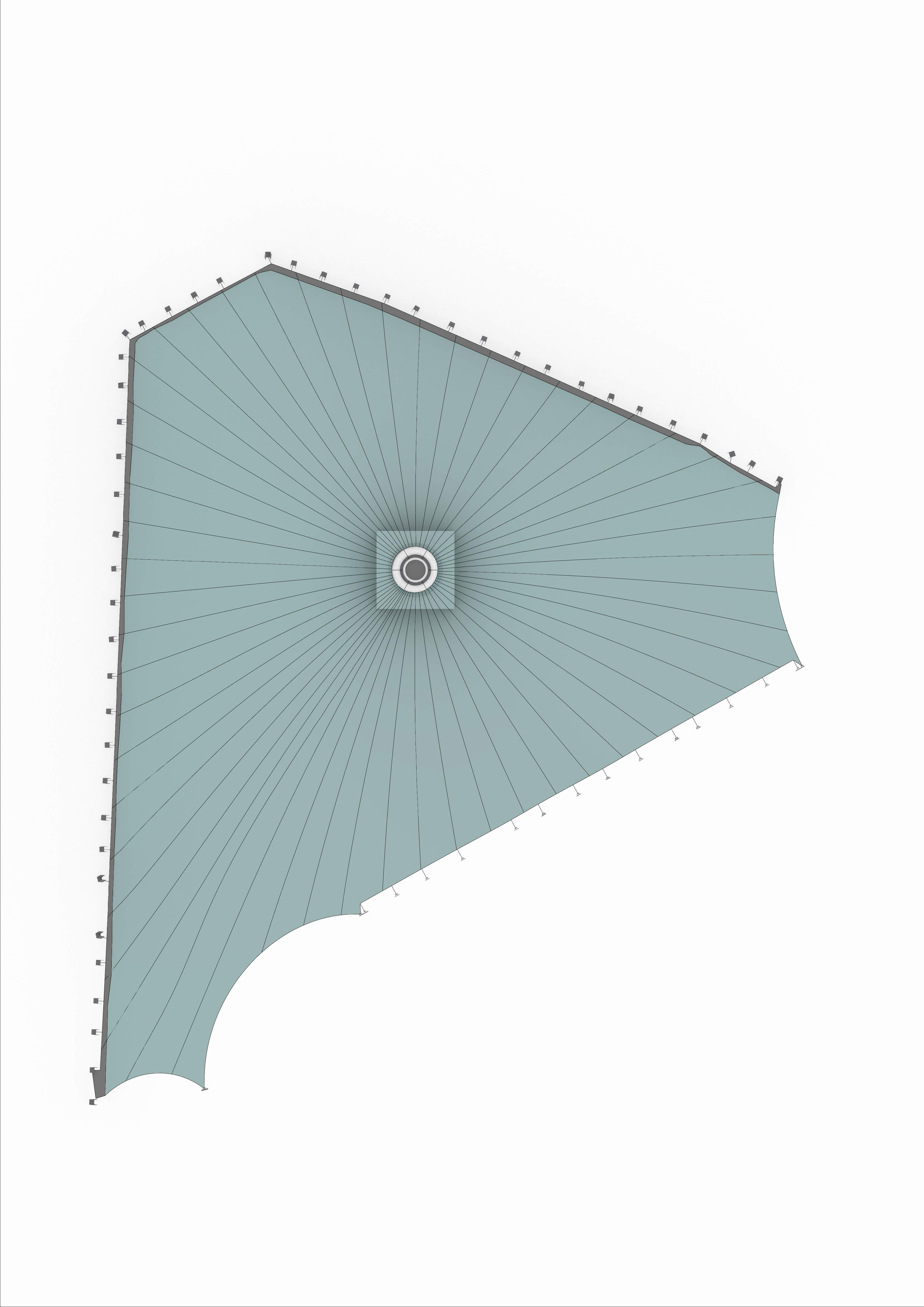
generate n radial construction lines
distribute them so that the spacing between neighbouring rays at the perimeter becomes as even as possible
This produces a geometrically stable radial order that can then be used to define control points and structure the next steps of the workflow.
In Rhino and Grasshopper terms, the method relies on a small number of core geometric operations:
checking whether a point lies inside a closed curve
generating rays from a reference point
intersecting those rays with a boundary curve
evaluating distance as a function of direction
redistributing the rays according to that directional distance field
These are exactly the kinds of custom geometric procedures for which the Grasshopper C# Script component is intended, and Rhino exposes the required geometry API through RhinoCommon.
Why a visual definition alone is not enough
A purely visual Grasshopper definition can easily draw radial lines. The difficulty lies elsewhere: the lines must not be spaced by equal angles, but by a weighted angular distribution that reacts to the changing distance from the internal point to the boundary.
That means the workflow is not just:
create lines
trim lines
display result
It is:
sample many directions
calculate first intersections
build a directional radius function
accumulate that function
redistribute the final set of rays
evaluate their spacing
That kind of repeated geometric evaluation is possible in visual Grasshopper, but it quickly becomes cumbersome. The C# component is useful here because it makes the logic explicit, compact, and repeatable. Grasshopper’s C# script component is specifically meant for custom algorithms embedded in a parametric model, with direct access to RhinoCommon geometry types and methods.
The geometric principle
The core idea is simple.
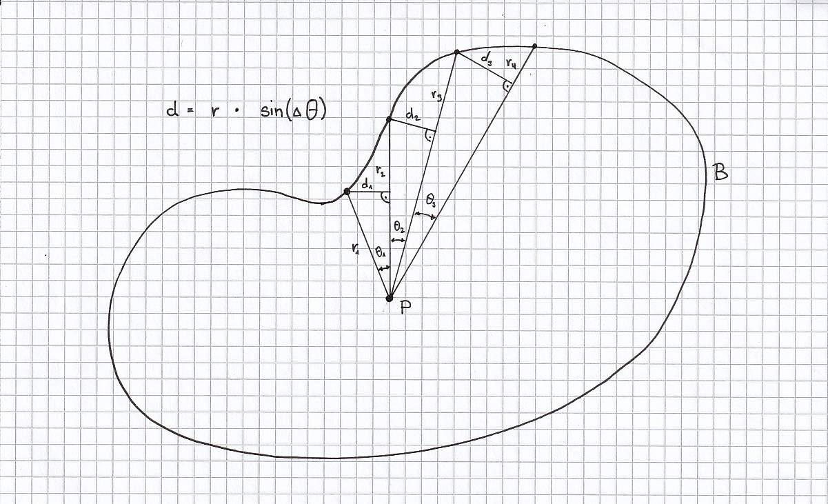
If two neighbouring radial lines enclose an angle Δθ, and the distance from the centre point to the boundary in that direction is r, then the local spacing at the perimeter is approximately proportional to:
d ≈ r · Δθ
So:
where r is large, Δθ must become smaller
where r is small, Δθ can become larger
This is why equal angular division fails for free boundaries.
The script therefore samples the boundary in many directions, measures the radial distance for each direction, and then redistributes the final rays using a cumulative weighting based on r. This produces a more balanced perimeter spacing than a simple equal-angle subdivision.
Rhino setup
The Rhino side is deliberately simple.
You need:
one closed planar boundary curve
one internal point P
one start point StartPt
The boundary can be a polyline, polycurve, or smooth curve, as long as it is closed. In RhinoCommon, point-in-region checks on curves are handled through Curve.Contains, which requires a closed curve region.
The start point does not have to lie on the boundary. It only defines the direction of the first ray. This is useful because the helper geometry often needs to align with a preferred seam direction, a construction axis, or a project-specific orientation.
Grasshopper setup
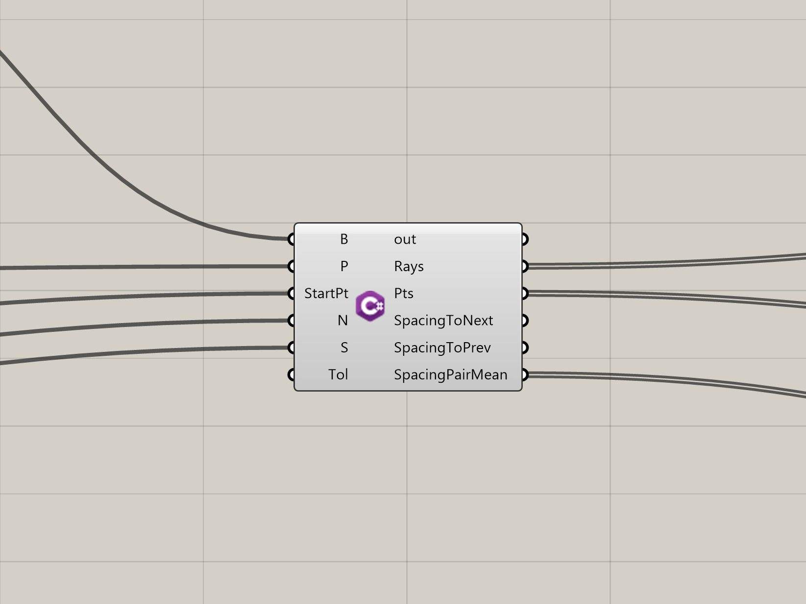
In Grasshopper, the inputs to the C# component are:
B → closed boundary curve
P → internal reference point
StartPt → point defining the first ray direction
N → number of final rays
S → number of angular samples for the scan
Tol → intersection tolerance
Recommended starting values:
N = 20 to 60, depending on panel count
S = 360 to 1440, depending on required precision
Tol = Rhino document tolerance or slightly above it
The outputs can be:
Rays → final radial helper lines
Pts → boundary end points of those rays
Angles → angular position of each ray
Spacing → one-sided perpendicular spacing to the next ray
SpacingMean → symmetric mean spacing between neighbouring rays
Why the start point matters
The start point is converted into a direction vector from P to StartPt. That vector is then projected into the plane of the boundary. The angle between the projected vector and the plane’s local X-axis defines the start angle.
RhinoCommon provides Vector3d.VectorAngle for measuring the angle between vectors in a given plane, which is exactly what is needed here.
This means the whole radial system can be rotated in a controlled way, while the weighted distribution logic remains unchanged.
The complete C# script
This is the full script for a Grasshopper C# component.
Inputs
Curve B
Point3d P
Point3d StartPt
int N
int S
double Tol
Outputs
object Rays
object Pts
object Angles
object Spacing
object SpacingMean
How the script works, step by step
1. Validate the geometry
The script first checks whether the boundary exists, whether it is closed, and whether the point P lies inside it. This is done with Curve.Contains, which evaluates the relationship between a point and a closed curve region.
If the point is outside the boundary, the whole radial logic breaks down, so the script exits immediately.
2. Build the start angle
The vector from P to StartPt is projected into the plane of the boundary. That projected vector becomes the reference direction for the first ray.
The angle between that vector and the plane’s X-axis is then calculated with Vector3d.VectorAngle. This gives the script a controlled rotational starting position.
3. Sample the boundary
The script does not jump straight to the final N rays. Instead, it first generates many test rays.
For each sampled direction:
a ray is cast from P
that ray is intersected with the boundary using Intersection.CurveCurve
the first valid intersection is selected
the radius from P to that point is stored
RhinoCommon’s Intersection.CurveCurve method is the key operation here. It returns the intersection events between the ray curve and the boundary curve.
The result is a discrete directional radius field.
4. Build the cumulative field
This is the crucial part.
The script does not redistribute the final rays by angle alone. It builds a cumulative weighting based on:
U = ∫ r dθ
In practical terms, this means the algorithm accumulates more “weight” in directions where the radius is larger. When the final target rays are distributed evenly across that cumulative field, more rays are allocated to larger-radius regions and fewer to smaller-radius regions.
That is what corrects the failure of equal angular spacing.
5. Interpolate the final ray angles
Once the cumulative field is built, the script places the final N rays at equal target positions in that field.
This is done by:
locating each target value inside the cumulative list
interpolating between the neighbouring sample angles
storing the resulting final angle
The final rays are then rebuilt from those interpolated angles and intersected with the boundary again.
6. Output spacing values
Finally, the script outputs spacing information.
Two values are useful:
Spacing = one-sided distance from the endpoint of ray i to the next neighbouring ray
SpacingMean = average of both one-sided distances between neighbouring rays
This is useful because the helper geometry may look visually regular while still containing local irregularities. The spacing outputs make that visible and measurable.
Why the spacing output matters
This is not only a display feature.
The spacing list makes it possible to:
test whether the distribution is sufficiently regular
compare different values of N
compare different start directions
judge whether the helper geometry supports a plausible panel sequence
In other words, the script does not only generate geometry. It also creates a way to evaluate that geometry.
Limits of the method
This should be stated clearly.
The script assumes:
a closed planar boundary
a valid internal point
a radial logic centred on that point
It is therefore well suited to funnel-shaped membranes, ring-supported surfaces, and other centrally organised geometries. It is not intended as a universal panelisation tool for arbitrary membrane types.
It is also important to repeat that the output rays are not the final cutting lines. They are a geometric scaffold. The actual cutting logic belongs to the later FEM and patterning stage.
Why this step matters in practice
For me, the relevance of this workflow lies in the fact that it turns an intuitive geometric idea into a reproducible method.
Instead of saying:
“the membrane should probably be divided radially”
the process becomes:
reconstruct the boundary
define the internal logic
generate a measurable radial order
pass that order on to the next digital step
That is precisely where parametric modelling becomes useful in textile architecture: not as a visual effect, but as a way to make intermediate design logic explicit.
Closing note
This script was developed as a way to clarify and stabilise a very specific step in a real project workflow. It sits between reverse engineering and pattern generation. In that position, it is neither form-finding nor final fabrication, but something in between: a geometric method for making the next step more reliable.
That intermediate zone is often where the real technical value of digital workflows lies.