The Question That Always Returns: Young’s Modulus

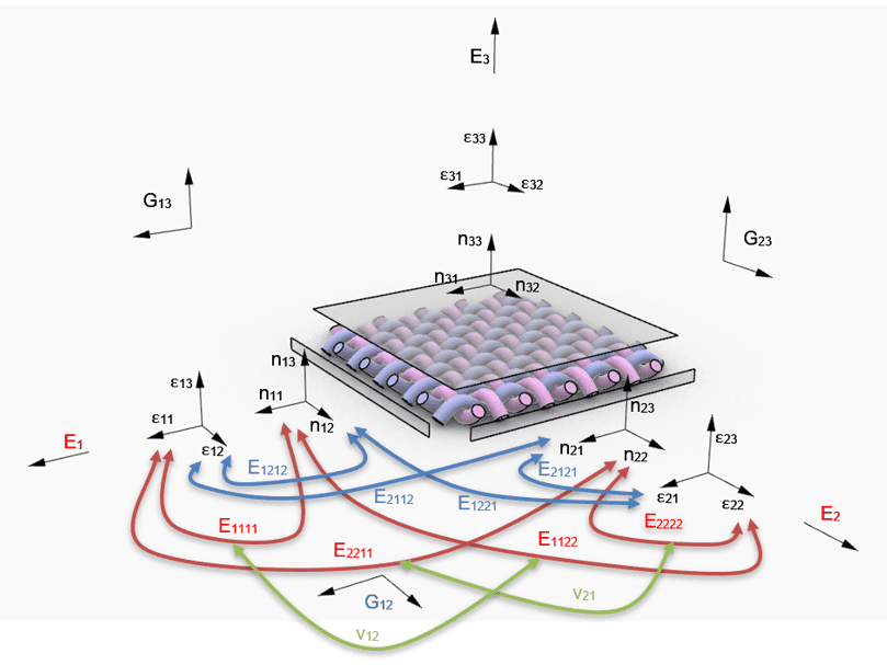
Why membrane stiffness is not a tabulated value – and what the biaxial test really tells us

“What Young’s modulus should I use?”

Anyone who works with the structural analysis of membrane structures will encounter this question sooner or later. It appears during studies, in project work, in FEM training, in conversations with engineers and often at precisely the moment when a model finally has to run under time pressure.

The question is understandable. Every numerical model needs input values. A material model needs stiffness values. For an isotropic material, one quickly thinks of Young’s modulus, shear modulus and Poisson’s ratio. For steel, aluminium or timber, there are established tabulated values, material classes, standards and calculation models. In many situations, one can choose a value, enter it and rely on the fact that this value has a clearly defined meaning within its intended field of application.

In membrane engineering, the situation is different.

Technical textiles are not conventional building materials. They are composite materials made of yarns, woven fabric, coating, adhesion layers and surface treatments. They are direction-dependent, load-path-dependent, time-dependent and non-linear in their deformation behaviour. Anyone who simply asks for “the” Young’s modulus is looking for a number where, in reality, a material state has to be understood.

That is where the difficulty lies – and also the fascination – of membrane engineering.

The question about Young’s modulus is not wrong. On the contrary, it is a valid question. But it is only the starting point. It immediately leads to deeper questions: Which material model is being used? Over which stress range is it supposed to apply? Which biaxial test is it based on? Which load paths were tested? Which values were actually derived from the test – and which had to be supplemented, assumed or checked for plausibility?

In membrane engineering, Young’s modulus is not a universal tabulated material value. It is a project-specific equivalent value within a defined range of prestress, loading and evaluation.

A personal perspective

My own view of this subject has been shaped by several tools. During my studies I worked with Formfinder, Rhino/Grasshopper, EASY and RFEM. For structural analysis, I used EASY and RFEM in particular. In my current professional practice, I mainly use RFEM for structural analysis.

This background influences the way I think. Nevertheless, this article is not about a particular piece of software. It is not a software manual, not an explanation of an input dialogue and not a promotion of any programme.

Software does not decide what the material is. It only decides in which language the material model has to be entered.

Some programmes work more directly with stiffnesses in warp and weft, with coupling, crimp or shear components. Other programmes translate this information into an orthotropic stiffness matrix. Others abstract certain values more strongly or handle them internally. The form of input may differ. The physical task remains the same:

How can the biaxial, orthotropic and load-path-dependent behaviour of a technical textile be described in such a way that a meaningful non-linear structural analysis becomes possible?

My understanding of this subject was shaped not only by software and project work, but also by lectures, teaching material and the continuous comparison with real membrane projects.

Intellectual foundations

The work and explanations of Rainer Blum, Heidrun Bögner and Rosemarie Wagner have had a significant influence on my understanding of material models for technical membranes. They provided important foundations, particularly in relation to biaxial material behaviour, stiffness matrices, compliance matrices and the evaluation of membrane materials.

Yet this understanding could not simply be adopted. It had to develop through my own engagement with calculations, comparisons, test evaluations, modelling and the continuous confrontation with real projects.

This article is therefore not merely a reproduction of literature. It is an attempt to make part of that path understandable.

Form-finding is not load analysis

At the beginning of many membrane structures stands form-finding. It is one of the essential particularities of textile construction. The form is not simply drawn and then checked. It emerges from boundary conditions, prestress and equilibrium.

In education, this idea is often described by the phrase “form follows force”. What is sought is an equilibrium figure that allows favourable load-bearing behaviour and a favourable distribution of membrane stresses. The form is therefore not freely selectable in the same way as with a bending-stiff component. It is the result of force equilibrium.

For classical form-finding, the real material model is initially not the decisive issue. Of course, a calculation programme needs a material model in order to compute. But the equilibrium form itself is primarily governed by geometry, boundary conditions, prestress, force densities, cables, edges and, where relevant, internal pressure.

This point is important because it gives some freedom in the early design stage. For initial form studies, the final project-specific tested material model does not necessarily have to be available yet.

At the same time, this point easily leads to a misunderstanding.

Because at the latest when structural load analysis begins, the situation changes fundamentally. As soon as self-weight, wind, snow, imposed loads, accidental actions, deformations, support reactions, edge forces or ponding are investigated, the material model is no longer secondary. The assumed stiffness then influences how the membrane deforms, how loads are redistributed, which membrane forces arise and which forces are introduced into the edge system, the primary structure and the supports.

Form-finding can therefore be largely independent of the real material behaviour. Load analysis cannot.

One could summarise it as follows:

For form-finding, a computationally functional material model may be sufficient. For load analysis, an engineeringly justified material model is required.

Why Young’s modulus is not enough

In practical analysis, complex material behaviour is often reduced to a few input values. A numerical model needs a describable stiffness. For orthotropic membranes, this means at least stiffnesses in warp and weft direction, coupling values or Poisson’s ratios, and a shear stiffness in the membrane plane.

But that does not solve the problem. It only moves it to the right place.

The programme can process the values entered. But it does not automatically know whether these values are meaningful for the specific material, load range, test history and project. This is where the actual engineering responsibility begins.

Coated fabrics are orthotropic. They behave differently in warp and weft direction. Their shear stiffness is usually low compared with their direct stiffnesses. And because of the non-linear behaviour of the material, there are no generally valid stiffness values for the simplified orthotropic linear-elastic replacement model that is often used in practice. The stiffness values must be derived from biaxial tests with stress ratios and load levels that correspond to the project.

This is a central point.

Young’s modulus is not a fixed material property here. It depends on the stress-strain state of the material. It depends on the level of prestress, the relationship between warp and weft, the loading history, the temperature, the duration of loading and the transverse contraction behaviour.

The material model therefore behaves like a mobile: when one parameter changes, all the others move with it.

Anyone who looks only for a single value does not see this mobile. They see only one point within a coupled system.

Programmes speak different languages

Different calculation environments describe the same physical problem in different ways. A specialist membrane programme may work with terms such as warp stiffness, weft stiffness, crimp stiffness, coupling stiffness or shear stiffness. A general FEM programme may formulate the same behaviour using an orthotropic stiffness matrix. A parametric model in Rhino/Grasshopper may initially approach the problem geometrically and process-wise before the structural analysis is carried out in another environment.

These differences are not insignificant. They can influence the way one thinks.

Those who come from matrix-based finite element modelling often think in terms of coefficients. Those who come from membrane-specific software tend to think in terms of warp, weft, prestress, load paths and cutting patterns. Those who come from geometric modelling first think in terms of form, boundary conditions and surface logic.

None of these views is wrong. But none of them is complete.

The material model does not lie in the input dialogue. It lies in the understanding of the relationship between material, load path, geometry and modelling assumption.

For this article, the decisive question is therefore not which programme is being used. The decisive question is whether one recognises what the programme requires from the user – and what it cannot know automatically.

From the complete material model to membrane idealisation

To understand the material model of a membrane, it is not helpful to begin immediately with the reduced plane model. Many models, formulae and software dialogues start at a point where the actual reduction has already taken place. One sees the input values, but no longer sees what the simplification refers to.

Especially at the beginning of an engagement with technical textiles, this can be confusing. One finds Young’s moduli, Poisson’s ratios, stiffness matrices and directional information, but the path from the spatial material reality to the plane membrane model often remains invisible.

For didactic reasons, it is therefore useful to begin by thinking more completely than is ultimately required.

A technical textile is initially not a two-dimensional calculation value, but a spatially built composite material. It has a warp direction, a weft direction, a material thickness, coatings, a textile structure and shear behaviour. In a complete material-scientific view, various directional stiffnesses, couplings and shear components can be considered.

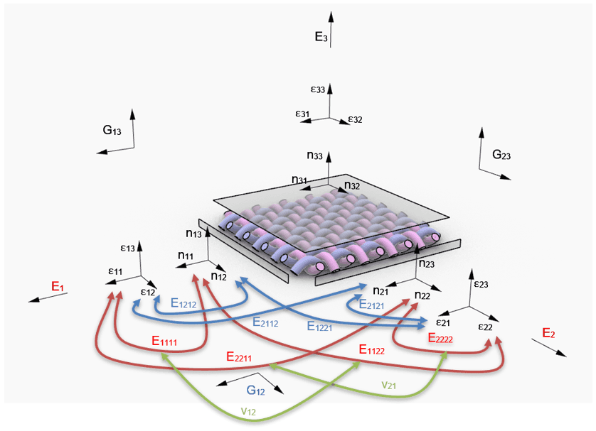
The indices 1 and 2 describe warp and weft direction; index 3 describes the thickness direction. The illustration deliberately shows more components than are later used in the membrane model. This makes visible which parts of the complete material understanding remain in the membrane idealisation, which are omitted and which are described only approximately.

In the illustration, a textile sample is deliberately placed at the centre. The warp and weft yarns are visible. The indices 1 and 2 may be understood as warp and weft. Index 3 represents the thickness direction. E₁​, E₂ and E₃​ are shown informatively as principal indices. The stiffness components are shown as links between the plane components. G₁₂​, G₁₃​ and G23​ also appear initially in the overall picture.

This representation is intentionally more complete than the later membrane model requires. That is precisely its value.

It shows that the reduction to a plane membrane model is not simply given. It has to be justified.

Direction 3, the material thickness, of course exists physically. It is by no means irrelevant for fabrication, weldability, keder details, folding behaviour, abrasion, ageing, weight or handling. For the global load-bearing behaviour of a classical membrane, however, it is not the governing structural direction.

A simple ratio illustrates this.

If the span of a sail is 20 m and the material thickness is about 1 mm, the result is:

From an engineering point of view, this is an extremely thin structure. The load-bearing behaviour is not described by a three-dimensional stress distribution through the thickness, but by membrane forces per unit length in the surface.

The membrane does not carry load through bending or compression in the thickness. It carries load through tensile forces in the surface.

The reduction of the material model is therefore not a simplification made for convenience. It follows from the load-bearing principle.

For the classical membrane description, the relevant plane components are primarily:

and

Normal strains and membrane forces arise in warp and weft direction. In addition, there is coupling between these directions. Loading in warp direction does not only produce strain in warp direction. It also affects strain in weft direction. Conversely, loading in weft direction acts back on the warp.

This is where transverse contraction becomes relevant. It is not a minor side effect, but part of the material model.

Coupling and decoupling of stiffness components

For the reduced plane membrane model, the essential components are the normal directions warp and weft, together with shear in the membrane plane. A more detailed formulation of the underlying material model can be found in the European Design Guide for Tensile Surface Structures. Rosemarie Wagner’s book Bauen mit Seilen und Membranen also treats this subject in a particularly clear way, especially the initial build-up of the matrix with normal and shear components and the subsequent reduction to the normal stiffnesses.

Before moving to the reduced engineering notation, it is helpful to look at a slightly more general in-plane formulation. In this form, the normal components and the shear components are still shown separately, and the tensorial shear strain components ε₁₂​ and ε₂₁​ are written explicitly. This makes the block structure of the material model particularly clear.

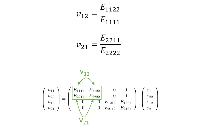
The upper-left block describes the coupling between warp and weft in the normal directions. The marked terms also show the definition of the directional Poisson’s ratios ν₁₂ and ν₂₁​. The lower-right block contains the in-plane shear terms. This representation is deliberately more general than the reduced engineering notation used later in the article.

In this more general notation, the in-plane stiffness relationship may be written as:

This matrix shows at a glance what is coupled and what is not. The normal components in warp and weft are connected through the off-diagonal terms E₁₁₂₂​ and E₂₂₁₁​. The shear terms, by contrast, form a separate block.

The corresponding component equations are:

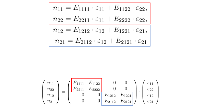
The normal equations form the coupled warp–weft block, while the shear equations remain in a separate block. This visual separation explains why the classical biaxial evaluation can determine the normal stiffnesses and coupling terms, but not the shear modulus directly.

For the engineering membrane formulation used in the following, the shear part is usually not written with two separate tensorial shear strain components. Instead, the tensorial components are combined into the engineering shear strain:

For the usual small-strain symmetric case, one has:

and therefore:

The plane stiffness relationship can then be written in the engineering notation used for the following discussion:

From the matrix, one obtains:

If tensorial shear strain ε₁₂​ is used instead of engineering shear strain γ₁₂​, the same shear relationship appears as:

This notation is important because it separates the roles of the individual components. E₁₁₁₁​ and E₂₂₂₂​ are stiffness coefficients of the normal matrix. E₁₁₂₂​ and E₂₂₁₁​ describe the interaction between warp and weft. E₁₂₁₂​ describes shear in the membrane plane.

For a symmetric elastic replacement model, one generally has:

and for the shear component:

The normal components may then also be written as:

with

and

This makes clear why the shear component does not follow from the normal equations for warp and weft. The coupling between n₁₁​, n₂₂​, ε₁₁​ and ε₂₂​ is described by E₁₁₂₂​ and E₂₂₁₁​. The shear component n₁₂ is described through E₁₂₁₂​, or G₁₂​. It is a separate material quantity.

There is an important distinction here that is easily overlooked: the matrix coefficients E₁₁₁₁​ and E₂₂₂₂​ are not automatically identical to the technical directional moduli E₁​ and E₂. As soon as there is coupling between warp and weft, the off-diagonal terms influence the effective directional moduli.

For the determinant of the normal stiffness matrix:

the technical directional moduli are:

For symmetric coupling with

the determinant becomes:

Only if there were no coupling between warp and weft, that is:

would one obtain:

and

In a real orthotropic membrane model, however, this coupling is an essential part of the material behaviour. E₁​ and E₂​ should therefore not be hastily equated with the matrix entries E₁₁₁₁​ and E₂₂₂₂​.

For the shear component, the relationship is more direct. If engineering shear strain is used,

and

then:

If tensorial shear strain ε₁₂​ is used instead, the same relationship appears as:

The material quantity remains the same; only the strain definition changes the notation.

For the evaluation of classical biaxial tests, this relationship is then reduced to the normal components:

This reduction is not arbitrary. It follows from the test. In a classical biaxial test, warp and weft are loaded and the strains in these two directions are evaluated. A true shear state is not generated and not measured.

This makes clear why the biaxial test provides the normal stiffnesses and the coupling between warp and weft, but not automatically the shear modulus G₁₂​. The shear component belongs to the plane membrane model, but remains outside the values directly determined by the reduced biaxial evaluation.

For the present discussion, this separation is crucial: the normal components in warp and weft are coupled; the shear component is separate.

This changes the way one looks at Young’s modulus. The question is no longer about a single value. It is about which parts of a spatially conceivable material model remain in the plane membrane model, which are omitted and which are described only approximately.

The controlled working range

If the real material behaviour of technical textiles is taken seriously, the material model can initially seem almost unmanageable. Non-linearity, viscoelasticity, transverse contraction, orthotropy, shear, creep, relaxation and load history all interact. A complete material-scientific description would hardly be manageable for many practical projects.

Practice therefore takes another path.

It does not try to represent every detail of the material behaviour in full. It limits the working range under consideration.

For PVC/PES membranes, it is often possible to linearise approximately within a controlled range of prestress and service loading. This does not mean that the material is fundamentally linear. It only means that the relevant portion of the stress-strain behaviour is described for calculation purposes as a linear replacement range.

The decisive point is that the membrane is not utilised arbitrarily close to failure. If the characteristic stress remains clearly below the tensile strength – in practice, an order of magnitude of around 25 per cent is often discussed – a working range is considered in which the behaviour may be sufficiently stable and interpretable for the numerical model.

This order of magnitude must not be misunderstood as a rigid rule. The decisive issue is not a single magic boundary, but the conscious limitation of the working range.

The membrane therefore does not become calculable because the material is simple.

It becomes calculable because the engineer deliberately limits the relevant working range.

The linearised replacement model does not claim that the material behaves linearly up to failure. It describes only one portion: the range between defined prestress and maximum service stress.

This limitation does not make verification unnecessary. On the contrary. Precisely because the model is a simplification, material strength, seam strength, connection details, edge zones, local stress concentrations, durability, serviceability, erection states and ponding must still be carefully checked.

But the approach explains why a linearised material model can work in practice: not because the material itself is linear, but because the structure is kept within a range in which this simplification is defensible.

The biaxial test as a material story

The next question is: where do the values for this replacement material model come from?

This is where the biaxial tensile test comes in, often carried out with a cruciform specimen. It is a central basis in membrane engineering for determining stiffness values and compensation values. The material is not tested only in one direction, but loaded in warp and weft direction. This corresponds much more closely to the actual state of a tensioned membrane than a simple strip tensile test.

But a biaxial test is not a table of values.

It is a description of material behaviour under a defined test procedure.

The biaxial stress-strain behaviour of coated fabrics is essential for structural engineering. The relevant quantities include stiffness in warp and weft direction, transverse extension and shear stiffness. At the same time, the numerical moduli are not constant. They depend on the applied force level and on the loading history.

This is also reflected in practical testing. Material stiffnesses under monoaxial and biaxial stress states can differ considerably and depend on the stress ratio between warp and weft. Typical biaxial tests use slit cruciform specimens with arms aligned parallel to the yarn directions and cyclic load protocols in order to reproduce different stress ratios and to condition the material.

The compact evaluation method used in Heidrun Bögner’s work illustrates this idea very clearly. In one load segment, one direction is cycled from prestress to the maximum service stress, while the other direction is held at the prestress level. From the strain gradients in warp and weft, compliance values are determined. The stiffness matrix is then obtained by inversion of the compliance matrix. The Poisson’s ratios are also defined from the stiffness components.

This is more than a calculation procedure. It shows that stiffness is read from a specific load window.

Young’s modulus is not simply present. It is derived from the behaviour of the material between two states.

For the evaluation of biaxial tests, the normal components are often written in matrix form:

with the inverse form:

In the first part of the loading programme, the weft direction is held at constant prestress while the warp direction is cycled from prestress to the maximum service stress. Thus:

For the stiffness formulation, this gives:

In the second part, the warp direction is held constant and the weft direction is loaded:

This gives:

In practical evaluation, the compliance formulation is often particularly intuitive. If one direction is held at a constant force level, the compliance can be read directly from the measured strain gradients. The stiffness matrix is then obtained by inverting the compliance matrix.

It is therefore not enough to look for the stated Young’s modulus in a test report. One has to know how the value was obtained.

Which prestress was applied? Which maximum service stress was selected? Which stress ratio between warp and weft was tested? How many cycles were carried out? From which cycle was the value evaluated? Was the loading or unloading branch considered? Over which strain interval was the gradient determined? Did the material come from the batch later used in the project? Was the test intended for structural analysis, for compensation, or for both?

Only when these questions are answered does the value become interpretable.

Young’s modulus is the result. The test procedure is the key to understanding it.

The missing part of the model: the shear modulus

With the biaxial test, important parts of the material model are described. But not all of them.

The shear modulus shows the limits of common practice particularly clearly.

A plane orthotropic membrane model needs, in addition to the normal stiffnesses in warp and weft and the coupling values between the two directions, a shear stiffness in the membrane plane:

In a more complete view, G₁₃​ and G₂₃​ may also appear. For the classical membrane plane, however, G₁₂​ is the relevant quantity. Shear components involving the thickness direction are not governing for the global membrane behaviour.

The problem is that G₁₂​ cannot automatically be obtained from a classical biaxial test used to determine the normal stiffnesses in warp and weft.

This is also visible in the reduced biaxial evaluation. The quantities evaluated are:

From these, compliance values are obtained and, subsequently, the stiffness matrix for the normal directions. A true shear component n₁₂​ or ε₁₂​ is not measured in this evaluation.

At the same time, shear behaviour is not irrelevant. Shear stiffness is one of the relevant properties of the biaxial short-term behaviour of coated fabrics. These values matter for the structural engineer, even though the numerical moduli are not constant and depend on force level and load history.

To determine the shear modulus, a separate test method is required, for example a bias-extension test or a shear-frame test. In the literature, shear behaviour is treated as an independent topic. Simplified test methods can be used to estimate shear stiffness by measuring angular change under transverse loading.

In practice, however, such tests are rarely carried out on a project-specific basis, at least in my experience. This creates a gap between test reality and calculation model.

The shear modulus is therefore an uncomfortable quantity: it is rarely tested in practice, yet often required by the numerical model.

Coated textiles usually do not have a particularly high shear stiffness compared with their normal stiffnesses. This softens the problem to some extent, but it does not make it disappear. Even if shear stiffness is often a smaller effect, it can influence stress concentrations in numerical analyses.

Especially in cases of large deformation, local distortion, corners, changes in cutting pattern direction or zones with strong directional changes, a high shear modulus may create additional stresses that would not occur with a very soft shear assumption. Conversely, a shear modulus chosen too low may underestimate local shear effects.

If no tested shear value is available, the shear modulus should therefore not be understood as a precise material value. It should be understood as a deliberately chosen model parameter. Its effect must be checked.

In practice, rough estimates are sometimes used, for example:

This is not a material-scientific derivation. At most, it is a rough estimate. It is also essential that units and programme definitions remain consistent. A value that seems plausible in one calculation environment cannot automatically be transferred to another formulation.

Another, equally approximate crutch consists of deliberately ignoring the decoupling of the shear modulus from the stiffness description and constructing a substitute value from the evaluated normal components:

This is not a correct calculation of the shear modulus. It is a crutch. An approximate value for an initial assessment.

It must also be clear whether tensorial shear strain ε₁₂​ or engineering shear strain γ₁₂ = 2ε₁₂​ is being used. Depending on the calculation formulation, the factor 2 may appear in a different place. This is precisely why such an approximation must not be transferred into a calculation model without checking.

Anyone working seriously with orthotropic membrane models should carry out calculation series with different G-values. The chosen value can, for example, be increased and reduced by 20, 40 or 60 per cent. Not in order to automatically obtain the “correct” value, but to develop a feeling for how sensitive the model is to G₁₂​.

The decisive issue is not only the absolute value. The decisive issue is whether the structure reacts sensitively to that value.

Existing biaxial tests as a basis for experience

Especially when dealing with projects by others or with older test reports, understanding the test procedure is essential. If the test procedure is unknown, the values can hardly be interpreted correctly. A Young’s modulus from an older project may be valuable. But it may also be misleading if the original load range, prestress level or stress ratio does not correspond to the new project.

Two biaxial tests on the same material can produce different equivalent stiffnesses without either of them being wrong. They may simply describe different load states.

This is also a major opportunity for practice.

Those who do not merely collect existing biaxial tests, but really read them, can build up experience. Over time, one begins to recognise how certain PVC/PES fabrics respond to prestress, which materials yield more strongly in weft direction, which materials show high initial strain, how pronounced the transverse contraction behaviour is and which stiffness assumptions are plausible for robust forms.

Such experience does not replace a project-specific biaxial test. But it allows rough assessments in early project phases. It helps in selecting a material, estimating tensioning paths, assessing bending-stiff edges, anticipating compensation and judging whether a form is likely to be robust or critical.

Existing biaxial tests are therefore not primarily lists of values.

They are reference cases.

They show how a material behaved under a specific load path. Those who know many such cases begin to develop a material feel. This material feel is not an alternative to testing. It is the prerequisite for reading tests correctly and making early decisions responsibly.

Conservative is not always conservative

A further point makes the choice of material model particularly demanding: in membrane engineering, there is no single conservative stiffness.

In conventional structures, it often seems natural to calculate with a higher stiffness. Higher stiffness means lower deformation, and lower deformation appears safe at first glance. For membrane structures, this way of thinking is dangerously incomplete.

A stiffer membrane generally leads to higher membrane forces. Edge cables, clamped edges, bending-stiff boundaries, the primary structure and the supports may also be loaded more strongly. For force verification, a higher stiffness can therefore be unfavourable.

For deformation checks, however, the opposite is often true. A membrane that is too stiff deforms less in the model. As a result, critical depressions, reversals of fall and possible ponding can be numerically softened or even hidden.

Ponding is one of the major risks in membrane structures. If a depression forms under snow, meltwater or heavy rain, water can collect in it. This additional weight increases the depression further. A self-reinforcing process develops.

This leads to a central statement:

In membrane engineering, there is no single conservative stiffness. There are only stiffness assumptions that are unfavourable for a particular verification.

For force checks, a stiffer model may be unfavourable. For ponding, a softer model may be unfavourable. For local shear effects, a higher shear modulus may again be critical. For other questions, it may create an overly stiff and unrealistic load distribution.

It is therefore not enough simply to choose a “safe” Young’s modulus. One has to understand which verification is being carried out and which assumption is critical for that verification.

From the test rig to the construction site

Material stiffness does not end with structural analysis. It reaches into fabrication and erection.

This is one of the reasons why membrane engineering cannot be neatly divided into isolated work packages. Material testing, form-finding, load analysis, compensation, cutting pattern generation, detailing, erection procedure and retensioning possibilities all interact.

Biaxial tests are used not only to determine elastic moduli, but also to determine compensation data. For this, the relevant load range has to be defined in relation to the project.

The biaxial test should also be carried out on the material actually used for the structure. The loading specifications for such tests should correspond to the prestress and governing membrane stresses in warp and weft direction obtained from the structural analysis. The remaining strains under prestress are then taken into account as compensation in the cutting pattern.

This makes clear that the biaxial test does not only provide input for structural analysis. It also provides information for the cutting pattern.

The membrane is not cut in its theoretical final shape. It is cut in such a way that, after erection, elongation and prestressing, it assumes the intended spatial form. The material model therefore directly connects analysis and fabrication.

Transverse contraction behaviour is also not merely an academic parameter. It can be decisive on site. If one direction of a mechanically tensioned membrane is stretched too early or too strongly, the transverse direction may appear to become too short. With flexible edge cables, some of this can still be accommodated. With bending-stiff edges, clamping profiles or fixed boundary lines, it can become critical. The membrane may then no longer fit the intended geometry, even if the cutting pattern was mathematically correct.

The problem is then not necessarily the cutting pattern.

It may lie in the tensioning path.

The practical literature on tensile surface structures repeatedly emphasises this link between design, fabrication and erection. The special mechanical behaviour of textile materials affects not only the calculation, but directly the manufacturability, erectability and quality of the completed structure.

Recovery behaviour is also important. Not every deformation that becomes visible during erection or use is immediately damage. Some deformations may partially recover, depending on material, temperature, load duration and stress state. Others remain as irreversible strain.

Initial strain determines which tensioning path is required until the membrane reaches its operational state. This is essential for detailing. A strongly curved form may place different demands on the system than a flat membrane surface. A material with high initial strain requires different tensioning paths and different reserves than a stiffer material.

Long-term strain, in turn, determines whether retensioning reserve is required, and how much. A retensionable edge is therefore not merely a constructive convenience. It may be the practical answer to creep, relaxation and irreversible strain.

The material model therefore does not only determine whether a numerical model works.

It influences whether a membrane can be fabricated, erected, tensioned and maintained in its intended form over time.

The small number and the larger whole

Seen in this way, Young’s modulus is only a small part of a much larger context.

It stands at the end of a chain:

Material batch → Biaxial test → Prestress level → Service load range → Evaluation → Material model → Non-linear analysis → Load analysis → Compensation → Cutting pattern → Erection → Service state

Each of these steps influences the others. This is why the material model in membrane engineering is not an isolated input in a software dialogue. It is a point of connection between the test rig, the calculation model, the workshop and the construction site.

This also explains why default values are problematic. They can be useful for first exercises, training sessions or rough preliminary studies. But they quickly create the impression that membrane stiffness is a general tabulated value.

It is not.

Those who adopt default values without understanding can produce a model that converges cleanly and produces plausible images – while still describing the real load-bearing behaviour only inadequately.

The real danger is not that a simplification is used. Simplifications are unavoidable in engineering.

The danger lies in no longer recognising the simplification as a simplification.

The real competence

The recurring question about Young’s modulus therefore remains valid. But it has to be asked differently.

Not:

What Young’s modulus does this membrane have?

But rather:

Which equivalent stiffness describes this material sufficiently well within the intended range of prestress and service loading?

And further:

• Which biaxial test does this value come from?

• Which load path was tested?

• Which prestress was applied?

• Which evaluation interval was used?

• Does the test correspond to the object?

• Which components were actually determined?

• How was the shear modulus dealt with?

• Which verifications are made conservative by this stiffness – and which may be beautified?

• What are the consequences for cutting pattern, erection and retensioning?

Only then does a numerical value become a material model.

Membrane engineering therefore requires more than software knowledge. It requires material understanding, experience, plausibility checks and the ability to translate between test report, calculation model, workshop and construction site.

Anyone who only asks for Young’s modulus is looking for a number.

Anyone who understands the biaxial test, the model reduction, the shear modulus and the tensioning path begins to read the material.

Note on foundations and sources

This article is based on my own practical and theoretical engagement with membrane structures, biaxial material testing, form-finding, non-linear analysis and cutting pattern compensation. It is not intended as a complete scientific treatise, nor does it attempt to represent all relevant publications, research work or experts in this field.

A significant part of my understanding was shaped not only by published literature, but also by lectures, teaching material and the way in which these topics were explained in an educational context. Particularly important for me were lecture materials by Rainer Blum, the course material Materials for Textile Architecture by Rainer Blum and Heidrun Bögner-Balz, and lecture material by Dieter Ströbel and Jürgen Holl. These materials provided an important basis for understanding the relationship between textile material behaviour, biaxial testing, form-finding and structural analysis.

The literature listed below has helped to reinforce, deepen and contextualise these foundations. In particular, the European Design Guide for Tensile Surface Structures, Rosemarie Wagner’s Bauen mit Seilen und Membranen, Heidrun Bögner’s work on stiffness evaluation, and Michael Seidel’s practical guide have remained especially relevant and accessible to me.

The formulae used in this article are based primarily on lecture material, on Bauen mit Seilen und Membranen and on the European Design Guide for Tensile Surface Structures. Some notations have been adapted, combined or supplemented for this article in order to make the relationships between stiffness matrix, compliance matrix, technical directional moduli and shear modulus more understandable.

The sources listed here should therefore be understood as the most important foundations of my own approach, not as an exhaustive bibliography. There are other publications, researchers and practitioners who address these topics with great depth and clarity. The selection reflects the sources and teachers that most strongly influenced my own path towards understanding the material model of technical membranes.

Sources and intellectual foundations

• Blum, R.: Lecture material on membrane structures, material behaviour and biaxial testing. Unpublished lecture material.

• Blum, R.; Bögner-Balz, H.: Materials for Textile Architecture. Lecture material.

• Ströbel, D.; Holl, J.: Lecture material on form-finding, analysis and construction of membrane structures. Unpublished lecture material.

• Forster, B.; Mollaert, M. (eds.): European Design Guide for Tensile Surface Structures. TensiNet, 2004.

• Wagner, R.: Bauen mit Seilen und Membranen.

• Bögner, H.: Stiffness Evaluation Equations. Working and lecture material.

• Seidel, M.: Tensile Surface Structures: A Practical Guide to Cable and Membrane Construction. Ernst & Sohn, 2009.

• Stranghöner, N.; Uhlemann, J. and others: contributions on material testing and the design of membrane structures, including publications in the Stahlbau-Kalender.

• JRC / European Commission: Prospect for European Guidance for the Structural Design of Tensile Membrane Structures.